Machine Learning in Bookmaking
Bookmakers have been using machine learning to manage their risks and set odds for sporting events but they have far more factors to consider than their customers. Bookmakers have to set their prices based not only on the probable outcome of a sporting event but also in reaction to how much money is being placed across a range of different bets as well as pricing competitively relative to other bookmakers.
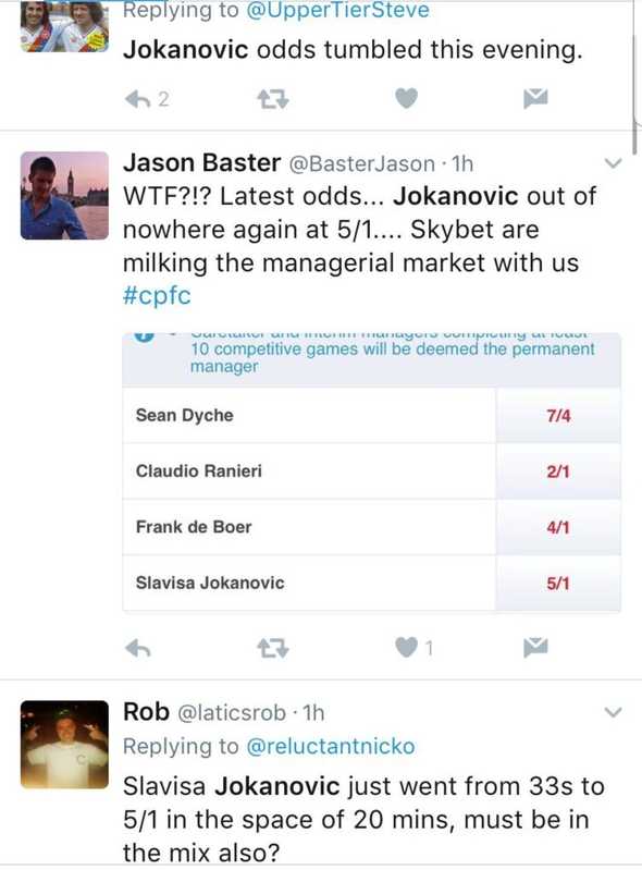
Often these decisions have to be made incredibly quickly. With the increased use of automation this can often be comparable to other types of financial trading. An interesting example of how quick bookmakers react to changes in market conditions was observed when I received an (incorrect!) tip on the next Crystal Palace F.C. Manager. In June 2017, after Sam Allardyce’s departure, the odds on Slaviša Jokanović to get the position were 33/1.
Because this was a relatively low volume market, a dozen bets from a handful of people caused the odds to drop to 9/1 in the space of about 30 minutes.
Interestingly, betting sites where no bets were placed responded by adjusting their prices on that market, while others didn’t respond at all. This is demonstrable of some bookmakers adjusting prices based on customer sentiment and competitors rather than factors that are causal in the outcome of a sporting event. This is a necessity for bookmakers, bets on Jokanović were a liability which wasn’t balanced on their book. The twittersphere also noticed the tumble in price!
While next manager markets are a difficult problem to solve with machine learning, boxing is less so. Boxing only involves 2 people (although coaches, promoters and cornermen are statistically significant), has fixed rules and there is a plethora of data available.
The dataset I was working with contained over 2 million fights. There were boxers in every weight class hailing from every corner of the world. Before I performed any feature engineering there were 28 variables to work with including; date of birth, date of debut, venue, stance and world ranking. However, some data was missing.
The Data
The dataset contained over 2 million fights and there were boxers in every weight class hailing from every corner of the world. Prior to conducting any feature engineering there were 28 variables to work with including; date of birth, date of debut, venue, stance and world ranking. However, some data was missing.
df.drop_duplicates(inplace = True)

null_columns=df.columns[df.isnull().any()]
df[null_columns].isnull().sum()
kopercentage 382
height 60958
draws 4
opponentwins 433
winmethod 1590
townofbirth 2948
worldrankingbyweight 6414
reach 117795
opponentlosses 15365
losses 4
opponentdraw 15365
countryrankingbyweight 7301Height and reach were the features where there was the greatest absence of data. The difference in your arm span and height are almost identical so it was possible to fill in the data where a boxer had only one of the variables available.
df['reach'] = df['reach'].fillna(df['height'])
df['height'] = df['height'].fillna(df['reach'])
Averages were taken across weight classes where other features with missing data was significant
Once the data had been cleaned, it was also necessary to ‘self-join’ the dataframe. Each record in the dataset represented one half of a fight. There would be a Boxer 1 and a Boxer 2. The target for each row would be Win, Lose, or Draw, with respect to Boxer 1. However, elsewhere in the dataset there would be a record for the same fight but with respect to the opponent. Duplicating the dataset, removing or renaming unnecessary columns and merging the two datasets back together allowed for a richer dataset without any repeated entries.
df2 = df

df2 = df2.drop(['boxerwin', 'winmethod', 'countryoffight', 'roundspath', 'division', 'sex', 'opponentwins', 'opponentlosses', 'opponentdraw', 'wins', 'losses', 'draws', 'totalboxersindivision', 'roundsinfight'], axis=1)

df2.columns = ('opponentkopercentage', 'opponentdebut', 'opponentboxrecrating', 'opponentheight', 'opponentrounds', 'opponentform', 'opponenttownofbirth', 'opponentworldrankingbyweight', 'name', 'opponentstance', 'opponentreach', 'opponentbouts', 'opponentcountryofbirth', 'opponent', 'opponentdob', 'venue', 'opponentcountryrankingbyweight', 'opponenttotalboxersindivisionandcountry' )

df3 = pd.merge(df, df2, on=['opponent', 'name', 'venue'])
Feature Engineering
Feature engineering is the process of using domain knowledge of the data to create features that improve machine learning algorithms. In this instance it was creating comparisons between the two fighters which might not be inferred automatically by the machine learning model during training. The new features I created included; difference in height, difference in reach and difference in their win records. Intunitively we know that a ‘home advantage’ is important in sports, so I added a binary feature which indicated whether the venue matched either of the boxers’ countries of birth.
#height diference
df3['Diff_height'] = df3.height - df3.opponentheight

#reach difference
df3['Diff_reach'] = df3.reach - df3.opponentreach

#name experience
df3['name_experience'] = df3.bouts - df3.opponentbouts

#opponent experience
df3['opponent_experience'] = df3.opponentbouts - df3.bouts

#name_win_pc
df3['name_win_pc'] = df3.wins / df3.bouts
df3.loc[df3.bouts == 0, 'name_win_pc'] = 0

#opponent_win_pc
df3['opponent_win_pc'] = df3.opponentwins / df3.opponentbouts
df3.loc[df3.opponentbouts == 0, 'opponent_win_pc'] = 0
The final step before feeding the data into a training model was to one hot encode all of the categorical variables. This is a necessary step as machine learning models need to compute numbers rather than text. The output of one hot encoding is a sparse matrix where each category is binarised – the matrix is populated with zeroes except the index of the matrix, which is marked with a 1.
Feature Importance
Prior to building a neural network I trained a random forest model to calculate the importance of each feature in my dataset. A feature importance chart provides a score that indicates how valuable a feature was in the construction of the decision trees within the model. The more a feature is used to make key decisions with decision trees, the higher its relative importance.
#Classifiers
from sklearn.ensemble import RandomForestClassifier

classifiers = [
    RandomForestClassifier(),
    RandomForestClassifier(bootstrap=True, class_weight=None, criterion='gini',
            max_depth=17, max_features=6, max_leaf_nodes=None,
            min_impurity_decrease=0.0, min_impurity_split=None,
            min_samples_leaf=1, min_samples_split=2,
            min_weight_fraction_leaf=0.0, n_estimators=70, n_jobs=1,
            oob_score=False, random_state=None, verbose=0,
            warm_start=True)

for item in classifiers:
    classifier_name = ((str(item)[:(str(item).find("("))]))
    print (classifier_name)

     Create classifier, train it and test it.
    clf = item
    clf.fit(feature_train, label_train)
    score = clf.score(feature_test, label_test)
    print (round(score,3),"\n", "- - - - - ", "\n")

importance_df = pd.DataFrame()
importance_df['feature'] = X2.columns
importance_df['importance'] = clf.feature_importances_

importance_df.sort_values('importance', ascending=False)
importance_df.set_index(keys='feature').sort_values(by='importance', ascending=True).plot(kind='barh', figsize=(200, 150))
Zoomed out you can see all the features and their importance relative to each-other. The top features ended up being;
- Difference in World Ranking
- Difference in Win %
- KO %
- The total number of rounds a boxer has fought in
- Age difference
On choosing which factors to include in a deep learning model I was hoping to find an strong inflection point which unfortunately wasn’t available. However, you can infer relative importance by comparing all the features to variables you know shouldn’t be statistically important. As draws are relatively rare in boxing and therefore shouldn’t be a high value feature in a decision tree, we can use the ‘draw’ feature as a yardstick and pick features to use in a deep learning model accordingly.
Neural Network
Using a relatively simple network architecture I was able to achieve an accuracy of 92% across the validation data using an 80:20 split. Further experimentation would include more complex architectures, dropout and batch normalisation but I was keen to use my model on future bouts.
classifier = Sequential()

classifier.add(Dense(output_dim = 6, init = 'uniform', activation = 'relu', input_dim = 40))

classifier.add(Dense(output_dim = 10, init = 'uniform', activation = 'relu'))

classifier.add(Dense(output_dim = 10, init = 'uniform', activation = 'relu'))

classifier.add(Dense(output_dim = 1, init = 'uniform', activation = 'sigmoid'))
Epoch 146/150
50886/50886 [==============================] - 31s 610us/step - loss: 0.1903 - acc: 0.9257
Epoch 147/150
50886/50886 [==============================] - 30s 581us/step - loss: 0.1902 - acc: 0.9259
Epoch 148/150
50886/50886 [==============================] - 30s 597us/step - loss: 0.1903 - acc: 0.9257
Epoch 149/150
50886/50886 [==============================] - 30s 580us/step - loss: 0.1901 - acc: 0.9253
Epoch 150/150
50886/50886 [==============================] - 28s 560us/step - loss: 0.1905 - acc: 0.9251I trained the neural network twice, once with the intention of picking whether or not a boxer would win and a second time with the intention of trying to pick which round the boxer would win in. The prices offered on picking the correct round are many magnitudes (often as high as 16/1) better than wagering on just a W or L outcome. The accuracy on training a round betting model achieved an accuracy of 17%. While this accuracy is poor, if you can afford to lose 83 times out of 100 but with a 5-16x return on successful bets, this may be a project worthy of further research.
Predictions
The output of the ‘win’ neural network was a decimal between 0 and 1. A score close to 0 indicated that the boxer in question had a low chance of winning, a score of 1 indicated a high chance of winning.
While you might consider this prediction enough to start placing your own bets it is first important to compare the confidence of your prediction to the implied probability offered by the bookmaker. Implied probabilities from fractional odds (the most common way of representing odds in the UK) are calculated using the following equation.
denominator / (denominator + numerator) * 100Once you have a probability from your model and an implied probability from the bookmaker you can set a decision threshold. Ideally you would refine your decision threshold by gathering large quantities of historical odds, compare them to the predictions of your model and then to the actual outcome.
In practice, this model favoured betting on clear favourites where the return on investment for an individual bet was less than 10%. Making a consistent 6-7% could have been achieved through automation but this was less interesting than scanning the book for ‘unicorn’ bets. These bets were advantageous to find as the offered odds were significantly mis-priced.
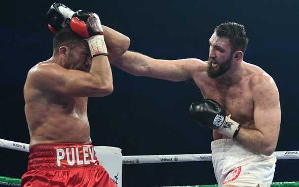
This happened in the bout between Hughie Fury and Kubrat Pulev in October 2018. Kubrat Pulev was a higher ranked boxer fighting on home turf in Sofia, Bulgaria. However, in British betting markets there was significant market sentiment in favour of Hughie Fury.
The machine learning model believed the probability of Kubrat Pulev winning the fight was 93%. The implied probability offered by the bookmakers was that he was only a marginal favourite at around 66% meaning I could place a high confidence bet at odds of 4/8.
The takeaway points for this project is that it is possible to engineer a small advantage over the bookmakers using machine learning. As the barriers to entry for learning about Artificial Intelligence are lowered, this is something that is available to more people every day.
With extra time and automation it may be possible to a get a moderate return on investment at a risk you can control by adjusting your thresholds for bet placement.
For those of you who are more casual betters, machine learning can be used to try and identify mis-priced bets. While I haven’t done any further research, I think mis-pricing and international betting markets would be an interesting area of research.
I will leave you with the odds offered on each round for Anthony Joshua to beat Joseph Parker in the UK…
Joshua to win in round 1    14/1
Joshua to win in round 2    10/1
Joshua to win in round 3    8/1
Joshua to win in round 4    8/1
Joshua to win in round 5    8/1
Joshua to win in round 6    8/1
Joshua to win in round 7    8/1
Joshua to win in round 8    9/1
Joshua to win in round 9    12/1
Joshua to win in round 10   14/1
Joshua to win in round 11   16/1
Joshua to win in round 12   20/1
and New Zealand…
Joshua to win in round 1    17/1
Joshua to win in round 2    15/1
Joshua to win in round 3    12/1
Joshua to win in round 4    12/1
Joshua to win in round 5    10/1
Joshua to win in round 6    10/1
Joshua to win in round 7    10/1
Joshua to win in round 8    12/1
Joshua to win in round 9    15/1
Joshua to win in round 10   17/1
Joshua to win in round 11   19/1
Joshua to win in round 12   21/1


